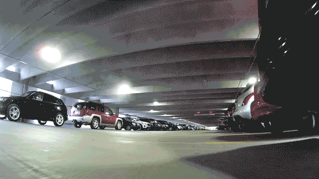
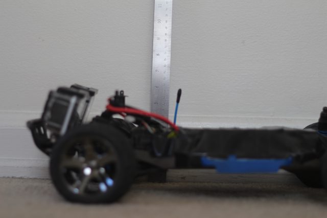
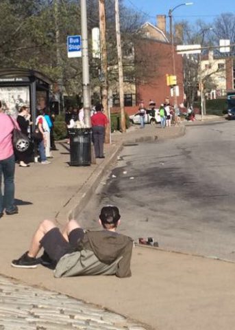
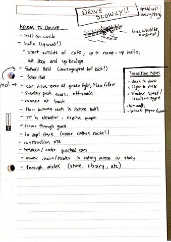
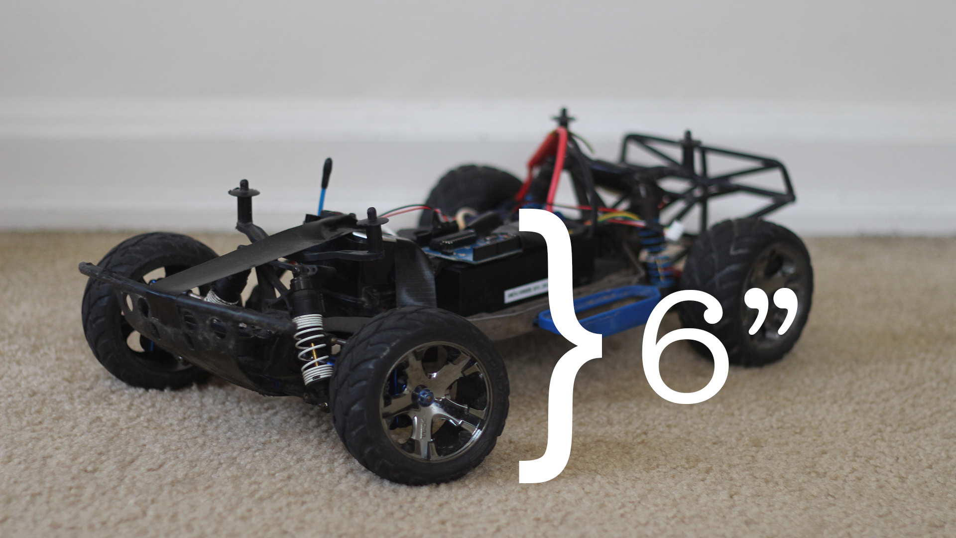
Little Car Scanning Underbellies of Big Cars
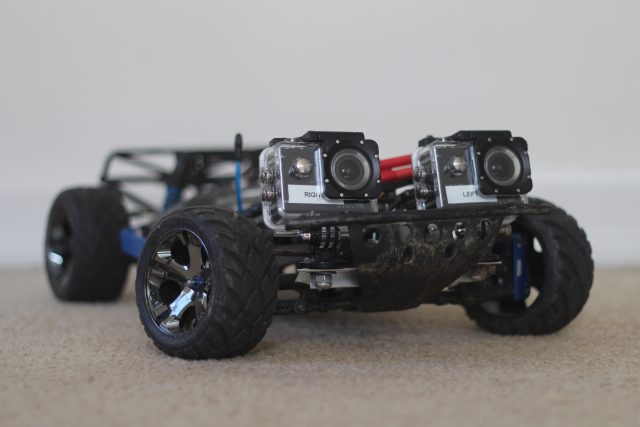
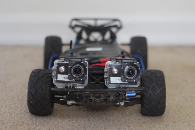
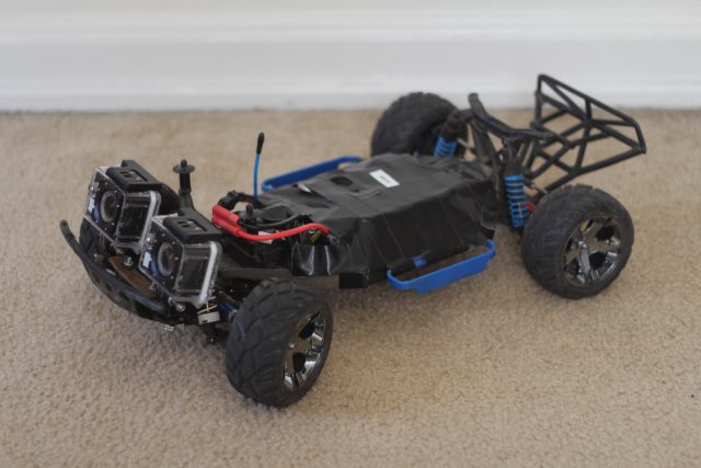
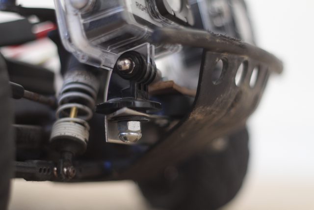
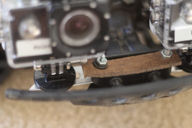
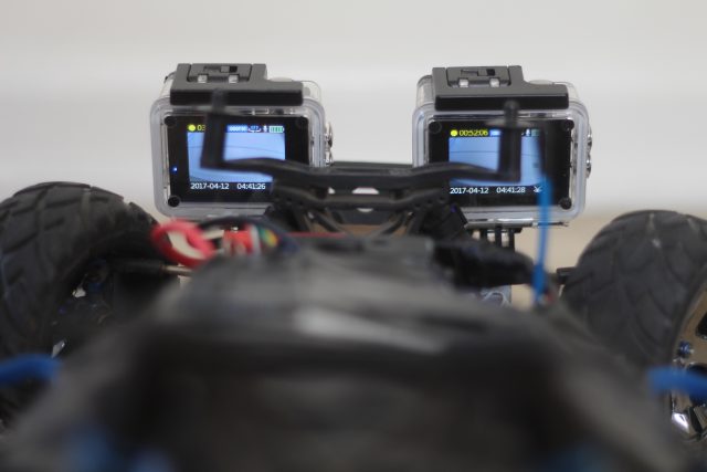
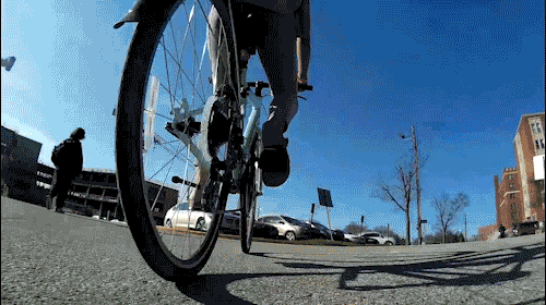
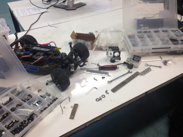
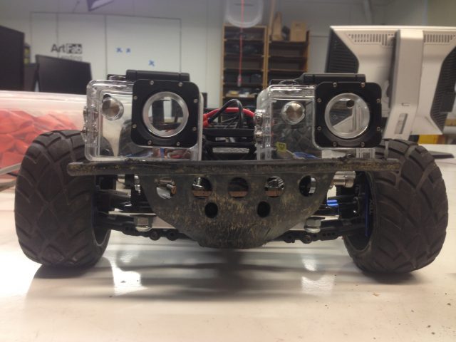
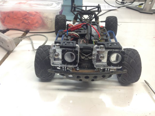
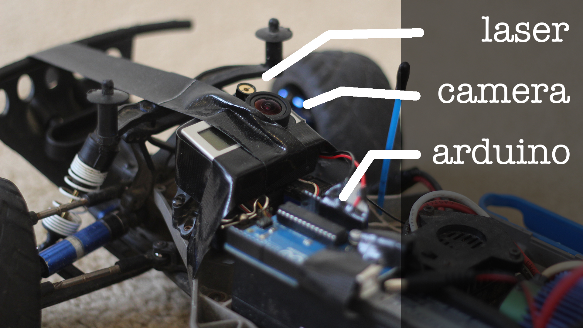
This little car is equipped with a line laser ($10 on Adafruit), a GoPro and an Arduino Uno.
When driven via remote control underneath vehicles at a constant rate of speed, capturing footage at 60fps, I am able to get an accurate reading of an approximately 1ft wide space of the underside of a vehicle, to be parsed into point-cloud data and eventually a 3D-printable model.

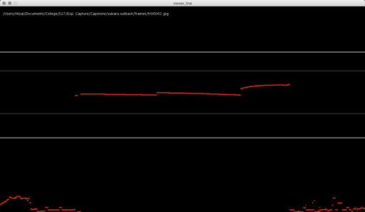
After experimenting with Photoshop and After Effects color-matching filters, I decided to write my own processing script to extract the laser’s path in the footage. I discovered it works best with footage shot in the dark, because it provided the cleanest and brightest result.
My script essentially tries to find the brightest and reddest color per column of pixels in the video. I also use averaging and other threshold values to “clean” unwanted data.
Processing: Analyze images for red laser path
String path = "/path/to/car/frames";
File dir;
File [] files;
//int f_index = 0;
PImage img;
//PVector[] points;
PVector[][] allpoints;
PVector[][] cleanpoints;
float[] frameAvgs;
float threshold = 30; // minimum red brightness
float spectrum = 75; // maximum distance from median

boolean debug = true;
boolean clean = false;
boolean pause = false;

int frame = 0;

void setup() {
  size(1280, 720, P3D);
  dir= new File(dataPath(path));
  println(dir);
  files= dir.listFiles();
  //points = new PVector[1280];
  allpoints = new PVector[files.length][1280];
  cleanpoints = new PVector[files.length][1280];
  frameAvgs = new float[files.length];
  convert();

  frameRate(30);
}

void convert() {
  for (int f_index = 0; f_index<files.length; f_index++) {
    String f = files[f_index].getAbsolutePath();
    PVector points[] = new PVector[1280];
    PVector fullpoints[] = new PVector[1280];
    while (!f.toLowerCase().endsWith(".jpg")) {
      f_index = (f_index + 1)%files.length;
      f = files[f_index].getAbsolutePath();
    }
    //text(f, 10, 30);

    img = loadImage(f);

    for (int x=0; x<img.width; x++) {
      PVector p = new PVector(x, 0, 0);
      float red = 0;
      float total = 0;
      for (int y=0; y<img.height; y++) { color c = img.get(x, y); if (red(c) > red && red(c) + green(c) + blue(c) > total) {
          red = red(c);
          total = red(c) + green(c) + blue(c);
          p.y = y;
        }
      }
      // check red threshold
      fullpoints[x] = p;
      if (red < threshold) {
        p = null;
      }
      points[x] = p;
    }

    // remove outliers from center
    float avg = pass1(points);
    frameAvgs[f_index] = avg;

    // remove outliers from median
    pass2(avg, points);

    allpoints[f_index] = fullpoints;
    cleanpoints[f_index] = points;
  }
}

void draw() {
  if (!pause) {
    background(0);
    frame = (frame + 1)%files.length;
    String f = files[frame].getAbsolutePath();
    while (!f.toLowerCase().endsWith(".jpg")) {
      frame = (frame + 1)%files.length;
      f = files[frame].getAbsolutePath();
    }
    text(f, 10, 30);
    drawLinesFast();
  }
}

public static float median(float[] m) {
  int middle = m.length/2;
  if (m.length%2 == 1) {
    return m[middle];
  } else {
    return (m[middle-1] + m[middle]) / 2.0;
  }
}

public static float mean(float[] m) {
  float sum = 0;
  for (int i = 0; i < m.length; i++) {
    sum += m[i];
  }
  return sum / m.length;
}

void keyPressed() {
  if (key == 'p') {
    pause = !pause;
  } else {
    debug = !debug;
    clean = !clean;
  }
}

// returns avg of points within the center
float pass1(PVector[] points) {
  float center = height/2-50;
  float sum = 0;
  int pointCount = 0;
  for (int i=0; i<points.length; i++) {
    if (points[i] != null &&
      (points[i].y < center+spectrum*2 && points[i].y > center-spectrum*2)) {
      sum += points[i].y;
      pointCount ++;
    }
  }

  return sum / pointCount;
}

void pass2(float avg, PVector[] points) {
  //float median = median(sort(depthValsCleaned));
  for (int i=0; i<points.length; i++) { if (points[i] != null && (points[i].y >= avg+spectrum
      || points[i].y <= avg-spectrum)
      && clean) {
      points[i] = null;
    }
  }
}

//void drawLines() {
//  background(0);
//  f_index = (f_index + 1)%files.length;
//  String f = files[f_index].getAbsolutePath();
//  while (!f.toLowerCase().endsWith(".jpg")) {
//    f_index = (f_index + 1)%files.length;
//    f = files[f_index].getAbsolutePath();
//  }
//  text(f, 10, 30);

//  img = loadImage(f);

//  for (int x=0; x<img.width; x++) {
//    PVector p = new PVector(x, 0, 0);
//    float red = 0;
//    float total = 0;
//    for (int y=0; y<img.height; y++) { // color c = img.get(x, y); // if (red(c) > red && red(c) + green(c) + blue(c) > total) {
//        red = red(c);
//        total = red(c) + green(c) + blue(c);
//        p.y = y;
//      }
//    }
//    // check red thresholdp
//    if (clean && red < threshold) {
//      p = null;
//    }
//    points[x] = p;
//  }

//  // remove outliers from center
//  float avg = pass1();

//  // remove outliers from median
//  pass2(avg);

//  // draw depth points
//  stroke(255, 0, 0);
//  strokeWeight(3);
//  for (int i=0; i<points.length; i++) {
//    if (points[i] != null)
//      point(points[i].x, points[i].y);
//  }
//  strokeWeight(1);

//  stroke(100);
//  //line(0, mean, width, mean);
//}


void drawLinesFast() {
  // draw depth points
  stroke(255, 0, 0);
  strokeWeight(3);
  if (clean) {
    for (int i=0; i<cleanpoints[frame].length; i++) {
      if (cleanpoints[frame][i] != null)
        point(cleanpoints[frame][i].x, cleanpoints[frame][i].y);
    }
  } else {
    for (int i=0; i<allpoints[frame].length; i++) {
      if (allpoints[frame][i] != null)
        point(allpoints[frame][i].x, allpoints[frame][i].y);
    }
  }
  if (debug) {
    float center = height/2-50;
    stroke(150);
    line(0, center-spectrum*2, width, center-spectrum*2);
    line(0, center+spectrum*2, width, center+spectrum*2);

    stroke(50);
    line(0, frameAvgs[frame]-spectrum, width, frameAvgs[frame]-spectrum);
    line(0, frameAvgs[frame]+spectrum, width, frameAvgs[frame]+spectrum);
  }
  //line(0, mean, width, mean);
}
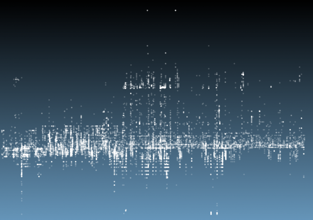
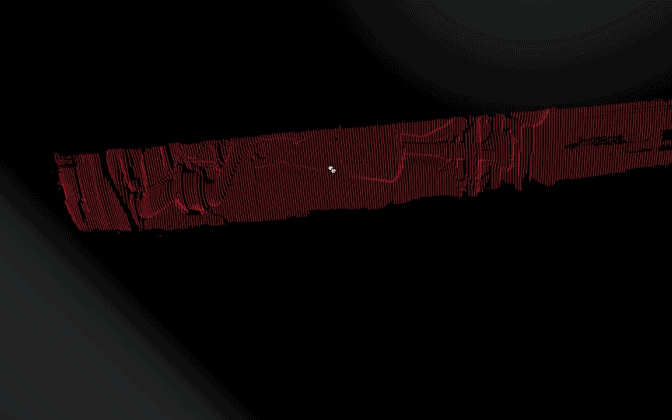
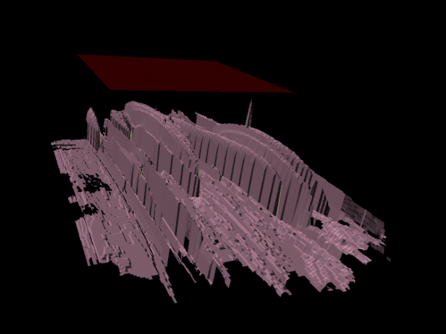
Once I got the algorithm down for analyzing the laser in each frame, I converted the y-value in each frame into the z-value of the 3D model, x was the same (width of video frame) and y-value of 3D-model to the index of each frame. The result looks like this when drawn in point-cloud form frame by frame:
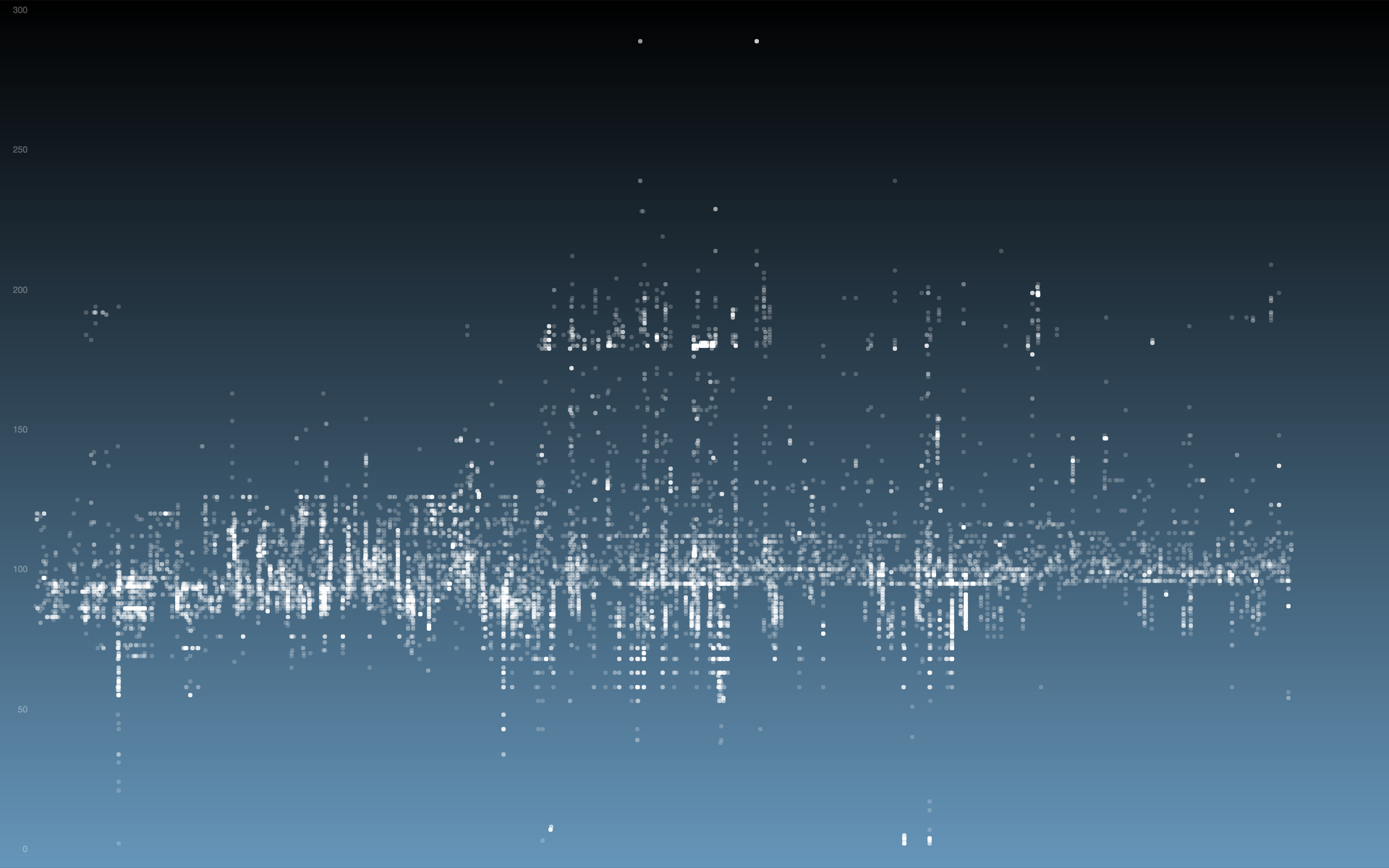
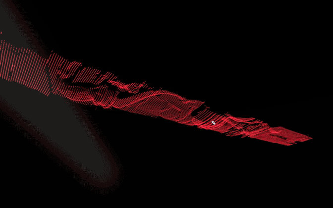
Thanks to some help by Golan Levin in drawing in 3D in processing, this is the same model when drawn with triangle polygons:
Processing: Analyze images for red laser path, create 3D point cloud
String name = "subaru outback";
String path = "/Path/to/"+name+"/";
File dir;
File [] files;
int f_index = 0;
PImage img;
PVector[] points;
PVector[][] allpoints;
float threshold = 30; // minimum red brightness
float spectrum = 75; // maximum distance from median

int smoothing = 1;
int detail = 1280/smoothing;
int spacing = 25;
float height_amplification = 4.5;

boolean lineview = true;
boolean pause = false;
int skip = 3;

int frameIndex = 0;

import peasy.*;
PeasyCam cam;

void setup() {
  size(1280, 720, P3D);
  surface.setResizable(true);
  //fullScreen(P3D);
  dir= new File(dataPath(path+"frames"));
  println(dir);
  files= dir.listFiles();
  allpoints = new PVector[files.length][detail];

  convert();
  //saveData();

  cam = new PeasyCam(this, 3000);
  cam.setMinimumDistance(10);
  cam.setMaximumDistance(3000);

  frameRate(30);
}

void draw() {
  if (!pause) {
    drawNew();
    frameIndex=(frameIndex+1)%files.length;
  }
}

void drawNew() {
  int nRows = files.length;
  int nCols = detail;
  background(0);
  noStroke() ;
  strokeWeight(1);
  //float dirY = (mouseY / float(height) - 0.5) * 2;
  //float dirX = (mouseX / float(width) - 0.5) * 2;
  float dirX = -0.07343751;
  float dirY = -0.80277777;
  colorMode(HSB, 360, 100, 100);
  directionalLight(265, 13, 90, -dirX, -dirY, -1);

  directionalLight(137, 13, 90, dirX, dirY, 1);
  colorMode(RGB, 255);

  pushMatrix();
  translate(0, 0, 20);
  scale(.5);
  fill(255, 200, 200);

  if (lineview) {
    noFill();
    stroke(255, 255, 255);
    strokeWeight(2);
    for (int row=0; row<frameIndex; row++) {
      beginShape();
      for (int col=0; col<nCols; col++) {
        if (allpoints[row][col] != null && col%skip == 0) {
          float x= allpoints[row][col].x;
          float y= allpoints[row][col].y;
          float z= allpoints[row][col].z;
          stroke(255, map(row, 0, nRows, 0, 255), map(row, 0, nRows, 0, 255));
          vertex(x, y, z);
        }
      }
      endShape(OPEN);
    }
  } else {
    noStroke();
    for (int row=0; row<(frameIndex-1); row++) {
      fill(255, map(row, 0, nRows, 0, 255), map(row, 0, nRows, 0, 255));
      beginShape(TRIANGLES);
      for (int col = 0; col<(nCols-1); col++) {
        if (allpoints[row][col] != null &&
          allpoints[row+1][col] != null &&
          allpoints[row][col+1] != null &&
          allpoints[row+1][col+1] != null) {
          float x0 = allpoints[row][col].x;
          float y0 = allpoints[row][col].y;
          float z0 = allpoints[row][col].z;

          float x1 = allpoints[row][col+1].x;
          float y1 = allpoints[row][col+1].y;
          float z1 = allpoints[row][col+1].z;

          float x2 = allpoints[row+1][col].x;
          float y2 = allpoints[row+1][col].y;
          float z2 = allpoints[row+1][col].z;

          float x3 = allpoints[row+1][col+1].x;
          float y3 = allpoints[row+1][col+1].y;
          float z3 = allpoints[row+1][col+1].z;

          vertex(x0, y0, z0);
          vertex(x1, y1, z1);
          vertex(x2, y2, z2);

          vertex(x2, y2, z2);
          vertex(x1, y1, z1);
          vertex(x3, y3, z3);
        }
      }
      endShape();
    }
  }

  //noFill();
  //strokeWeight(10);
  //stroke(0, 255, 0);
  //fill(0, 255, 0);
  //line(0, 0, 0, 25, 0, 0); // x
  //text("X", 25, 0, 0);

  //stroke(255, 0, 0);
  //fill(255, 0, 0);
  //line(0, 0, 0, 0, 25, 0); // y
  //text("Y", 0, 25, 0);

  //fill(0, 0, 255);
  //stroke(0, 0, 255);
  //line(0, 0, 0, 0, 0, 25); // z
  //text("Z", 0, 0, 25);

  popMatrix();
}

void convert() {
  for (int f_index = 0; f_index < files.length; f_index++) {
    points = new PVector[detail];
    String f = files[f_index].getAbsolutePath();
    while (!f.toLowerCase().endsWith(".jpg")) {
      f_index = (f_index + 1)%files.length;
      f = files[f_index].getAbsolutePath();
    }

    img = loadImage(f);

    for (int x=0; x<img.width; x+=smoothing) {
      PVector p = new PVector(x, 0, 0);
      float red = 0;
      float total = 0;
      for (int y=0; y<img.height; y++) { color c = img.get(x, y); if (red(c) > red && red(c) + green(c) + blue(c) > total) {
          red = red(c);
          total = red(c) + green(c) + blue(c);
          p.y = y;
        }
      }
      // check red threshold
      if (red < threshold) {
        p = null;
      }
      points[x/smoothing] = p;
    }

    // remove outliers from center
    float avg = pass1();

    // remove outliers from median
    pass2(avg);

    // draw depth points
    for (int i=0; i<points.length; i++) {
      if (points[i] != null) {
        //point(points[i].x, points[i].y);
        float x = i - (detail/2);
        float y = (f_index - (files.length/2))*spacing;
        float z = (points[i].y-height/4)*-1*height_amplification;
        allpoints[f_index][i] = new PVector(x, y, z);
      } else {
        allpoints[f_index][i] = null;
      }
    }
  }
}

// returns avg of points within the center
float pass1() {
  float center = height/2-50;
  float sum = 0;
  int pointCount = 0;
  for (int i=0; i<points.length; i++) {
    if (points[i] != null &&
      (points[i].y < center+spectrum*2 && points[i].y > center-spectrum*2)) {
      sum += points[i].y;
      pointCount ++;
    }
  }
  return sum / pointCount;
}

void pass2(float avg) {
  for (int i=0; i<points.length; i++) { if (points[i] != null && (points[i].y >= avg+spectrum
      || points[i].y <= avg-spectrum)) {
      points[i] = null;
    }
  }
}

void keyPressed() {
  if (key == 'p')
    pause = !pause;
  if (key == 'v')
    lineview = !lineview;
}
I then exported all the points in a .ply file and uploaded them to Sketchfab, which all models are viewable below (best viewed in fullscreen).
Volvo XC60
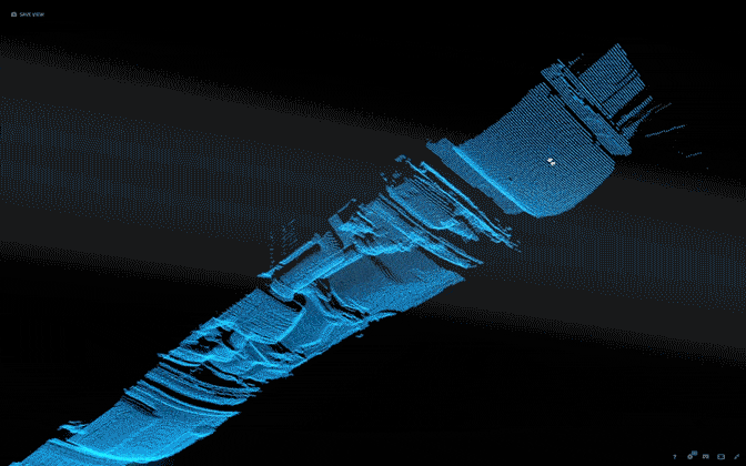
Subaru Outback
The resolution is a bit less because the car was driven at a higher speed.
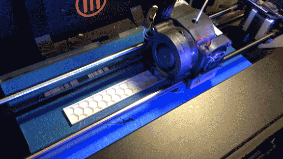
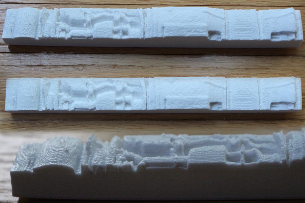
3D Print
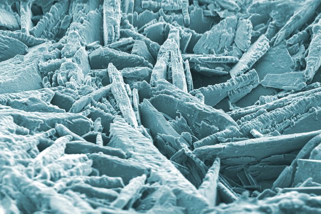
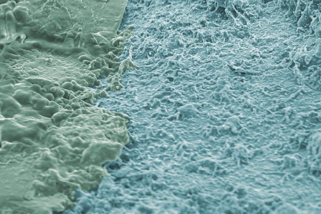
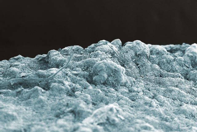
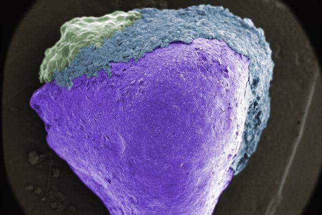
As a final step in this process, I was recommended to try 3D printing one of the scans, which I think turned out amazing in the end! There were a few steps to this process. The first was to fill in the gaps created from missing point data in the point cloud. I approached this in two different ways-first I used an average of the edges to cut off outliers. Then I extended the points closest to the edge horizontally until they reached the edge. And lastly, any missing points inside the mesh would be filled in using linear interpolation between the two nearest points on either side. This helped create a watertight top-side mesh. Then with the help of student Glowylamp, the watertight 3D model was created in Rhino and readied for printing using the MakerBot. The following are the process and results of the 3D print.
Special Thanks
Golan Levin, Claire Hentschker, Glowylamp, Processing and Sketchfab
ISSUES
I had a few hiccups along the development of this app. The first was, embarrassingly enough, mixing the width and length values in the 3D viewer, resulting in this which we all thought was correctly displaying the underside of a vehicle, somehow:
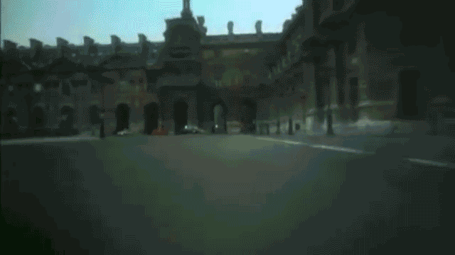
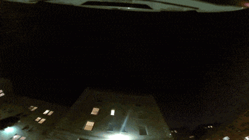
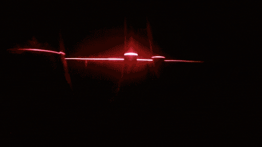
The other issue was the various forms of recording under vehicles. The following footage is the underside of a particularly shiny new Kia Soul:
Which resulted in a less-than-favorable 3D point cloud render:
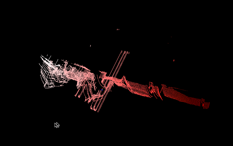
There are also plenty of other renders that are bad due to non-ideal lighting conditions.